Fast Monte Carlo Ticker Permutation w/ Pandas
This post details how using native Pandas operations gives significant speedup over a naive implementation in the context of permuting price paths.
Motivation
Lately, I’ve been looking into how to perform more rigorous backtests for my trading indicators.
The main source of my study is Permutation and Randomization Tests for Trading System Development by Timothy Masters. The book details methodologies for estimating strategy performance such as permuting existing price data to form multiple alternate paths, allowing us to run our strategy on multiple possible realities.
Suppose we want to generate one of these walks for our asset \(S\) from time \(t_0\) to \(t_n\) which moves as \(S_0, S_1, ..., S_n\). \(S_i\) can be Microsoft’s closing price at day \(i\) as an example.
The movement of the asset can be modelled as a small multiplicative modifier \(\sigma\) where \(S_0\cdot\sigma_0=S_1\) and \(S_0\cdot\sigma_0\cdot\sigma_1=S_1\cdot\sigma_1=S_2\) (assuming \(\sigma\) comes from a normal dist. gives us a geometric brownian motion, handy for basic pricing + modelling).
The rest of this post assumes that we work w/ log pricing as this makes the movement additive and gives the benefit of normalizing price differences over long horizons.
Under log pricing, our new equation for asset movement is then \(S_n = S_0 + \sigma_0 + \sigma_1 + ... + \sigma_{n-1}\). Notice how reordering the \(\sigma\)’s doesn’t change the final price as the movements are commutative.
We can obtain \(S_3\) from (\(S_0 + \sigma_0 + \sigma_2 + \sigma_1\)) or (\(S_0 + \sigma_2 + \sigma_1 + \sigma_0\)) despite them being separate paths.
As such, we can generate nearly any number of alternate paths that start at \(S_0\) and end at \(S_n\) by reordering \(\sigma\). The book details why we want to do this, but as a TL:DR, path permutation destroys patterns and preserves trends.
Naive Implementation
Here’s a basic implementation of the path permutation algorithm in Python.
Note 3 key differences in the implementation vs the explanation:
- the
Close,HighandLoware moved relative to the dailyOpento preserve intraday trends - we permute
Open->Close->Opento preserve interday trends rather thanClose->Close - we permute interday and intraday movements separately to break up predictable patterns
def get_example_data():
    import yfinance as yf
    df = yf.download(['MSFT'], period='10y', auto_adjust=True)
    df.columns = ['Close', 'High', 'Low', 'Open', 'Volume']
    return df

def get_perm_slow(log_df, seed=None):
    log_perm_df = np.log(copy.copy(log_df))
    # intraday relative movements of high, low, close relative to open
    # keep first bar constant or else first and last bar won't be identical
    intra_h_o = (log_df['High'] - log_df['Open'])[1:]
    intra_l_o = (log_df['Low'] - log_df['Open'])[1:]
    intra_c_o = (log_df['Close'] - log_df['Open'])[1:]
    # shift(-1) is next row val, shift(1) is prev
    inter_c_o = (log_df['Open'].shift(-1) - log_df['Close'])[:-1]

    # keep price of first bar stable
    np.random.seed(seed)
    perm_ids = np.random.permutation(list(range(0, len(log_df)-1)))
    perm_ids2 = np.random.permutation(perm_ids)

    log_perm_df = pd.DataFrame(columns=['Close', 'High', 'Low', 'Open'])
    log_perm_df.loc[0] = copy.copy(log_df.iloc[0])

    # starting from first bar
    for idx in range(len(log_df)-1):
        pidx = perm_ids[idx]
        pidx2 = perm_ids2[idx]
        # new open = last Close + permuted inter-bar movement
        o = log_perm_df['Close'].iloc[-1] + inter_c_o.iloc[pidx]

        # h,l,c = new open + permuted log inter diff
        h = o + intra_h_o.iloc[pidx2]
        l = o + intra_l_o.iloc[pidx2]
        c = o + intra_c_o.iloc[pidx2]

        log_perm_df.loc[len(log_perm_df)] = [c, h, l, o]

    log_perm_df.index = log_df.index
    return log_perm_df
It gets the job done, but runs fairly slowly averaging .51 seconds per call on a 10 year chunk of OHLC data.
Back to the drawing board
We want this code to run thousands of times per strategy, meaning we want to squeeze more performance. The bottleneck is the for loop recreating the price path by going through each movement in a random order.
We can greatly expedite this process if we can find a way to write that loop using Pandas operations, and letting the library handle the optimization.
The for loop can be broken down into two operations:
- get a new
Openby adding interday movement from the lastClose - get
High,LowandCloseby adding intraday movement relative toOpen
Careful reading of the code + algorithm shows that we can perform these updates independently w/ vectorized calls as long as we take care to propagate the Close -> Open shift properly.
High and Low are intraday movement relative to Open and rely on Close, so we can trivially vectorize their movement relative to the Open.
# Old
for idx in range(len(log_df)-1):
    pidx2 = perm_ids2[idx]
    h = o + intra_h_o.iloc[pidx2]

# New
x['High'] += intra_h_o.iloc[perm_ids2].to_numpy()
Open only depends on the intraday movement from the last Close so we don’t need to modify it.
Intraday Close movement is trickier and requires 2 vectorized operations:
- Add the permuted movement of
Closerelative toOpenas a cumulative sum (eachClosemovement permanently affects every subsequentClose) - propagate this movement to every subsequent bar except
Close(intradayCloseupdate lags by 1 timestep to every other bar)
Lastly, we add the interday movement from Close to Open using the same trivial vectorization as the High and Low bar, except we use a cumulative sum to propagate the movement to subsequent rows.
Better Implementation
Putting all of this together gives us the following code.
def get_perm(log_df, seed=None):
    np.random.seed(seed)
    # decouple intraday bar from interday shift
    perm_ids = np.random.permutation(list(range(0, len(log_df)-1)))
    perm_ids2 = np.insert(np.random.permutation(perm_ids) + 1, 0, 0)

    x = pd.DataFrame(0.0, index=range(len(log_df)), columns=['Close', 'High', 'Low', 'Open'])
    x.index = log_df.index

    intra_h_o = (log_df['High'] - log_df['Open'])
    intra_l_o = (log_df['Low'] - log_df['Open'])
    intra_c_o = (log_df['Close'] - log_df['Open'])
    inter_c_o = (log_df['Open'].shift(-1) - log_df['Close'])[:-1]

    #  Don't move first bar
    intra_h_o.iloc[0] = 0
    intra_l_o.iloc[0] = 0
    intra_c_o.iloc[0] = 0

    start = log_df['Close'].iloc[0]
    x += start

    x.loc[x.index[0], :] = x.loc[x.index[0], :].combine_first(log_df.iloc[0])

    # Intraday permute
    x['High'] += intra_h_o.iloc[perm_ids2].to_numpy()
    x['Low']  += intra_l_o.iloc[perm_ids2].to_numpy()
    x['Close'] += intra_c_o.iloc[perm_ids2].to_numpy().cumsum()

    # Propagate close movement to future bars
    propagate_close = np.concatenate([[0], intra_c_o.iloc[perm_ids2].cumsum()[:-1]])

    # Already updated Close, other bars lag update by 1
    cols_to_update = x.columns.difference(['Close'])
    x.iloc[1:, x.columns.get_indexer(cols_to_update)] += propagate_close[1:, None]

    # Interday permute
    x = x.add(np.concatenate([[0], np.cumsum(inter_c_o)]), axis=0)

    return x
We’ve replaced the for loop with vectorized operations allowing Pandas to optimize the code using its backend framework (NumPy).
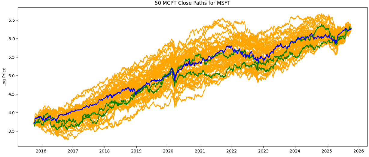
In my testing, the faster implementation gives > 200% speedup, and is able to run the example in ~.002 seconds rather than 0.51.
An example of some permuted Close paths for the last 10 years of MSFT is shown below.